Strategies for analysing quasi experimental data

9.33 The issues to be considered when analysing the data obtained in a study mirror those which arise at the policy design stage: identifying a comparison group and addressing selection bias. Indeed, if the policy is designed appropriately, many of the potential problems will have already been addressed. This sub-section revisits those issues from the standpoint of the tools used for analysing the data. Once again, technical details of these tools are provided in supplementary guidance.

9.34 Impact evaluation is often carried out in combination with a process evaluation. It is helpful to draw on contextual information to understand what the data truly represent. For example:

• What is meant by "treatment" in the context of the policy, and how might outcomes plausibly unfold over time as a result?

• Are the outcomes being analysed valid measures of the policy's aims? Have there been any changes in the way information is recorded that could have influenced the results?

• Was the policy implemented as intended? Are there any special cases or exceptions to be aware of?

9.35 Regression modelling plays a central role in the analysis of experimental and quasi-
experimental data. Regression provides estimates of association between two or more variables, and whether that association is "significant" in the sense of being expected to exist in some wider population as opposed to just having arisen by chance in the data at hand. A regression output in isolation, however strong the "significance", is silent on the question of whether the association is causal. So the fact that there is a "significant policy effect" is not necessarily evidence that the policy caused any change to occur. (Further technical detail on regression is provided in supplementary guidance.)

9.36 Whether the analyst can go further, and infer that the policy did cause the change,
depends on the context of the study. It is valid to do so if an effective random allocation scheme was used: the data are then described as "experimental". More often than not, however, allocation will not be random. What the analyst then requires is a strategy for using the observational (that is, non-experimental) data to approximate an experiment - known as an identification strategy (Box 9.F).

Box 9.F: Questions to guide an identification strategy

9.37 The first part of the strategy involves finding one (or more) comparison groups. Ideally, the design of the policy allocation will already have provided one. Usually, the comparison group will be a group of actual subjects (people, institutions or areas). If no actual group can be identified then the comparison group might be a forecast or projection (but see paragraph 9.49).

9.38 The strategy next has to consider whether the comparison group is equivalent - that is, whether it is a plausible match for how the treatment group would have looked had it not received the treatment. For example, if the comparison group consisted of individuals who did not participate in treatment for purely administrative reasons, such as non-availability of a caseworker at the right time, it could be regarded as "as good as random" because the administrative reasons for non-participation are unrelated to the characteristics of the individuals.

9.39 Provided some basic conditions are met, control groups from RCTs, and equivalent comparison groups as defined above, provide an estimate of the counterfactual "as-is" and analysis might be relatively simple. Ideally it might only involve conducting a t-test15 comparing the figures for the outcome of interest for the two groups; a significant difference is interpreted as evidence of a policy effect. Even in these simple cases, though, the analyst should always examine the assumptions critically in the way described in the next sub-section. If data are available on additional factors thought to affect the outcome, even if they are not sources of selection bias as such, then it is worthwhile to include these additional factors in the model. This is true for all the models discussed here, not only for RCTs. Doing so improves the power of the design.

9.40 If the groups are thought to be non-equivalent, further steps must be taken to modify the model in a way that will allow any apparent policy effect to be attributed to the policy, just as it would be for a true experiment. This means overcoming selection bias as introduced in paragraph 9.14. More specifically, selection bias arises when there are factors (Box 9.G) affecting both:

1 the likelihood of an individual being exposed to the policy; and

2 the outcome measure, other than via exposure to the policy.

9.41 For example, the level of motivation of an individual to obtain a job could affect both his likelihood to enrol on a job training programme but also how likely he would be to gain employment in the absence of the programme. So a simple comparison of programme participants with non-participants would not be a valid basis on which to evaluate the impact of the programme.

Box 9.G: Factors leading to selection bias

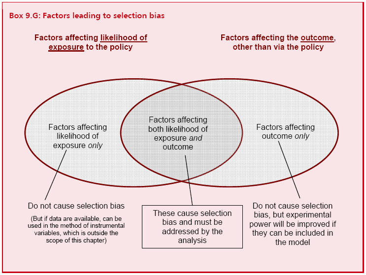
9.42 Factors which affect only one out of (1) and (2) above, or which affect neither of them, do not bias the results. This points to a strategy for reducing or even eliminating selection bias. If all the factors affecting likelihood of selection are known about - as might be the case if the policy had objective selection criteria - then they can be adjusted for, in one of the ways outlined below. This will be sufficient to cover everything in the intersection region of the Venn diagram in Box 9.G, and explains why accurate knowledge of the policy allocation criteria is so valuable to the researcher¹⁶ (A similar strategy could be applied if all the factors affecting the outcome were known about, but this is rarer and requires very rich data.)

9.43 The next case to consider is when policy allocation is neither fully random (as in an RCT) nor fully deterministic (as in an RDD or other objective scheme). It is this middle ground that is often encountered, because the criteria leading to exposure to the policy may not be fully known to the researcher - perhaps because they involved a subjective element, either on the part of the intervention provider or the participant. The question then to consider is whether, after adjusting for factors known to affect allocation, there are grounds for believing that whatever variation in exposure remains is "as good as random". If this is a reasonable assumption then a comparison after adjusting for these factors can proceed as in the deterministic (RDD-style) case.

_________________________________________________________________________
15 Note that a t-test may be regarded as a special case of a regression analysis: it can always be formulated as a regression model with appropriate use of dummy variables.

16 Within this framework, the regression discontinuity design (paragraph 9.22) may be seen as a special case of perfect objective allocation. By definition, all the factors affecting exposure are known about, because they are encapsulated in just one variable - namely the assignment score. This is what makes the RDD so effective in addressing selection bias.