7.1 The Trade-Off Between Investment and Maintenance
To analyze the trade-off between investment and maintenance, let us consider a twice-repeated and slightly modified version of our basic procurement model. To focus on the operator's incentives to invest, we assume that the firm gets a basic stock of infrastructure to run off public service on G's behalf at date t = 1. Improving this stock requires some extra investment which costs  today but this pays off tomorrow in terms of lowering operating costs by an amount a. Another strategy would be to avoid incurring any initial investment and then cutting operating costs with more maintenance.
Costs in each period are respectively given by:
| and |
|
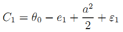
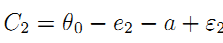
where the operating cost uncertainty εi (i = 1,2) is normally distributed with zero mean and variance σ2, and ei is maintenance effort undertaken at date ei.31
Investing increases accounting costs in the short-run but, because of a positive externality between design and operation, reduces the long-run cost of the service.32 Implicit in our formulation is the fact that the cost of investment is not observable to G meaning that it is (at least partly) aggregated with other costs, noticeably the first-period operating costs, in the firm's book.33
Finally, and consistently with Section 3, we assume that the stock of new investment has a social value b0 + ba with b > 0. In practice, this simply means that there is a difference between the social and the private returns on investment. Assuming that investment is verifiable, its first-best level satisfies: aFB = 1 + b whereas a = 1 would be privately optimal.
For simplicity, there is no discounting.
• Non-Verifiable Investment: Let us turn now to the case where the investment a is non-verifiable and must be induced by G through designing adequate incentives. Denote ti(Ci) = αi - βiCi the cost-reimbursement rule used at date i34 Let us first consider the case where G can commit himself to such a two-period contract {t1(C1), t2(C2)}.
Still assuming a quadratic disutility of maintenance effort in each period, the firm chooses its whole array of actions (a*, e1*, e2*) to maximize its long-run expected payoff:
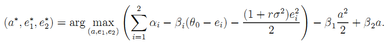
This leads to the following incentive constraints:
| (22) |
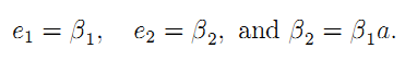
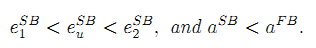
An interesting benchmark is obtained when G offers the stationary contract with slope βuSB, i.e., the contract that would be optimal in the absence of any concern on the renewal of the infrastructure. This contract induces a stationary effort e1 = e2 = βuSB and an investment level, namely a = 1, which is privately but not socially optimal as soon as b > 0. There is too little investment in renewing infrastructure with such stationary contract. Raising this investment requires modifying the intertemporal pattern of incentives.
Result 11 Assuming full commitment to a long-term cost-reimbursement rule; the optimal longterm contract entails higher powered incentives towards the end of the contract than at the beginning and an ineffcient level of investment:
The intuition behind this proposition is straightforward. To boost the firm's incentives to undertake a non-verifiable investment, G must let F bear less of the costs and enjoy most of the benefits associated to that investment. This is best achieved by offering cost-plus contracts in the earlier periods and fixed-price contracts towards the end of the relationship.35 Still, this is not enough to align the private incentives to invest with the socially optimal ones and underinvestment follows.
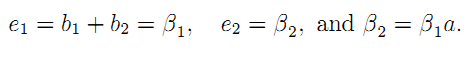
Remark 3: History-dependent contracts. Let us suppose now that G can commit himself to two-period history dependent contract {t1(C1), t2(C1, C2)} where t(C) = α1 - b1C1 and t2(C1,C2) = α2- b2C1 - βC2. The benefit of considering this larger class of incentive schemes is well-known since Rogerson (1985), pushing part of the rewards for a good cost realization in the first period towards the second one improves the trade-off between risk and incentives in this first period.36 To see how and to check the robustness of our earlier results, observe first that, given the history-dependent contract above, the agent chooses his effort array (e1, e2, a) so that:
| (23) |
For a given incentive intensity β1 the risk borne by the agent over the two periods is better spread when half of those incentives are pushed to the second period, i.e., when 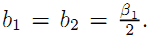 Everything happens as if the first period variance on costs was lowered by one half. This implies high-powered incentives to reduce costs in the first period and an unambiguously increase in welfare. But, this welfare improvement has a detrimental impact on investment which becomes less attractive than improved maintenance.
Remark 4: Non-stationary environments. Learning about operating costs over time could be modeled by allowing the noise on the firm's maintenance effort to diminish over time. This effect also goes towards having higher powered incentives in later periods of the relationship which boosts incentives to invest.
Similarly, in the case of a growing demand, having growing operating costs in the second-period may also call for greater returns on maintenance as time goes on. This non-stationary contract also requires higher powered incentives in later stages which boosts investment.
Remark 5: Ownership transfer. It is straightforward to extend the framework above to the case where the firm would enjoy some residual value when owning the asset during the life of the contract. Using the notations of Section 3.3, this would amount to introduce a residual value worth  sa with s ≠ 0 (whereas our analysis above has supposed s = 0). Of course, there is still not enough investment because of the hold-up problem ex post. However, private ownership still boosts incentives to invest and is thus complementary to a shift of second-period contracts towards fixed-prices.
Remark 6: On-going investments. Consider the case where the effect of a new investment depreciates over time. The power of the incentive scheme must decrease over time to optimally trade off incentives and risk insurance. As investments have been made earlier in the past, the firm will rely more on maintenance to keep operational costs low.
_____________________________________________________________________________________________________
31 In full generality, we could allow uncertainty on operating costs to be time-dependent. In particular, we might give particular attention to the case σ2 < σ1 which means that uncertainty on operating costs may decrease over time (due for instance to learning by doing and better assessments of performances).
32 With respect to Section 3.3, the investment a has no impact on the social value of the assets which remains fixed and equal to b0.
33 In this respect, our formulation differs from that in Section 2 where the cost of the quality-enhancing effort was off the book.
34 Decomposing the agent's rewards into two different incentive schemes in each period makes presentation somewhat easier especially in view of the no-commitment case that will be analyzed later on. Of course, this class of incentive schemes entails a loss of generality since, contract t2(C2) does not depend on the first period realization of costs which makes it impossible to use history dependent contracts whose value in dynamic incentive problems is well-known (see Remark 3 below). Alternatively, one could view the overall intertemporal incentive scheme  PA as being offered upfront by the government with all payments being made at the end of the period once the whole realizations of all first- and second-period costs are then known.
35 In a model that departs from modeling any incentive issues, Goncalves and Gomes (2007) show that a private operator may have an incentive to boost his maintenance effort towards the end of the concession length to meet a predetermined target.
36 History dependent contracts can also help to address adverse-selection problems. In Lewis and Sappington (1997), for example, the power of the incentive scheme decreases with early performance to reduce agent's incentives to understate ability in the first period.