2.1  Triangular

The triangular distribution is the most common distribution used to quantify risks that are assumed to be continuous random variables, but that cannot be defined as a normal distribution. A triangular distribution has one peak and uses the following three parameters to determine the expected value of the cost outcome of each risk:

•  Maximum

•  Most likely

•  Minimum

The maximum scenario represents the most unfavourable outcome associated with a risk event. The most likely scenario, or mode, is the most likely consequence of a risk event and the minimum scenario represents the least severe outcome possible for a risk event.

In addition to specifying maximum and minimum amounts, confidence levels can be used to express the degree of certainty associated with these events. For example, an estimated maximum value of $100,000 for a triangular distribution can be made at the 95 per cent confidence level, meaning that values higher than $100,000 are possible but have no more than a five per cent chance of occurring.

Expressing estimates in terms of confidence intervals is useful for risk work, as individuals tend to be more comfortable providing estimates at 95 per cent, which means that one time out of 20 they will be incorrect, rather than being asked to say with 100 per cent certainty what a maximum value might be. This is particularly true as one moves towards the maximum tail of a distribution where values can increase rapidly. Asking for 100 per cent certainty can result in a very high maximum value, even if it is highly unlikely to happen (i.e., less than five per cent).

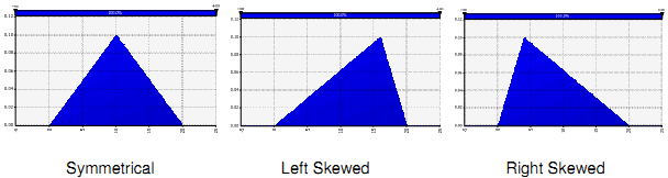
Triangular distributions will often be skewed meaning that, unlike symmetrical distributions, the values are not equally distributed about the mean and the most likely risk outcome will be closer to either the minimum or maximum values. In a right-skewed distribution there are more, very large values that result in a long tail after the peak when the curve is drawn from left to right. For example, a distribution for the risk of construction delays typically has a long right tail because more things are expected to go worse than planned rather than better, resulting in costly delays that generate greater cost for this risk. A left-skewed distribution has a greater number of very small cost values, relative to the median and mode, resulting in the tail appearing before the peak. Examples of triangular distributions, both symmetrical and skewed are shown in Figure 8.

Figure 8:  Triangular distribution forms

Given a probability distribution for a particular risk, statistical software such as @RISK or Crystal Ball can be used to determine the expected value of that risk. In cases where the distribution is symmetrical, the expected value of each risk will be equal to the most likely scenario. For risks that are asymmetrical, or skewed, the expected value must be determined with the assistance of statistical software.

An example of the inputs and expected value for a skewed triangular distribution are summarized below in Figure 9.

Figure 9:  Summary of Risk inputs and outputs for a triangular distribution

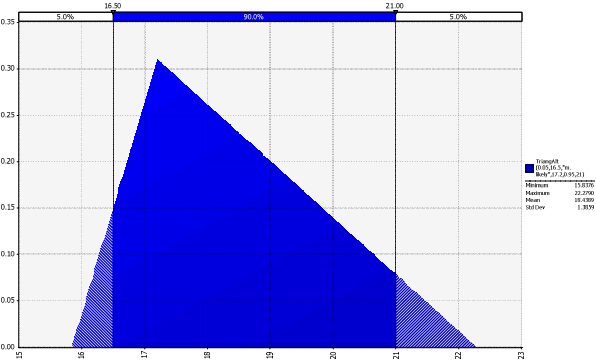
Example (Risk 1)

The price of cement is changing rapidly and there is 90 per cent probability that the price will be somewhere between $16.5 and $21.0 per 100 pounds for the next four years. Given that the price of cement will change, the most likely price during next four years is estimated to be about $17.2 per 100 pounds. The expected price of the cement using statistical software is $18.4:

Figure 10: @Risk Distribution Diagram for Risk 1