2.2 Discrete
A discrete distribution is the second most common distribution used for risk quantification, and is the preferred method for quantifying risks with discrete (i.e., separate and individual) outcomes.
A discrete distribution relies on the assumption that risks are independent of each other, so that the occurrence of one risk will not affect the occurrence of another. A discrete distribution function can have multiple peaks, with the highest one representing the most likely outcome. Although the discrete distribution is not as simple as a triangular distribution to define due to its higher number of inputs and requirement of a 100 per cent confidence interval, the inputs for the discrete distribution can be as easily obtained during a risk workshop as those for triangular distributions.
Defining discrete distributions relies on the experience of the project team to determine estimates of the magnitude of consequence and probability of occurrence for a particular risk event. The project team determines a number of outcome points-usually three, but any number equal or greater than two can be used. For each potential outcome a probability of occurrence must be assigned that are often characterized as high, medium, and low in relation to the severity of consequence. The high scenario would represent a severe outcome with a significant cost consequence. The medium scenario would represent a moderate outcome, with a less severe cost consequence, and the low scenario would correspond to an even smaller consequence with different cost consequence assumptions associated with it.
The expected value of a discrete distribution can be calculated using a simple formula or with statistical software. The simple formula is:

Where:
|
| = Expected value of risk |
|
| = Probability of the risk event occurring |
|
| = Probabilities of i-th outcomes (Note: sum of all probabilities equals 1) |
|
| = Cost consequences of i-th outcomes |


Figure 11: Summary of Risk inputs and outputs for a Discrete Distribution
|
| Likelihood (Probability of cost impacts) | Cost of Consequence | Expected Value | |||||||
| Risk | Probability | P1 | P2 | P3 | P4 | C1 | C2 | C3 | C4 |
|
| 2 | 35% | 20% | 45% | 35% | 0% | $80 | $140 | $180 | $0 | $49.70 |
| 3 | 65% | 40% | 15% | 20% | 25% | $100 | $150 | $220 | $250 | $109.85 |
Following are two simplified examples of discrete distributions.
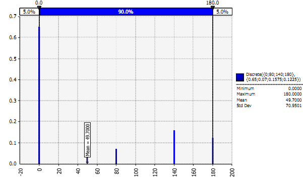
Example (Risk 2)
A project team responsible for a bridge the Ministry of Transportation and Infrastructure wants to build over a river, estimates that there is 35 per cent probability that the project design will need to be altered during the procurement process. Given that project design must be altered, there is a 20 per cent probability that the changes are minor and the resulting increase in the design cost will be only $80; however, there is 45 per cent chance that changes will be more significant and will cost $140. There is also 35 per cent chance that the changes are major and will cost $180. The expected value of this particular risk is $49.70, calculated as follows:
 = 35% x { 20%($80) + 45%($140) + 35%($180)} = $49.70
The discrete distribution for Risk 2 is shown in Figure 12. The figure shows the shape of the discrete probability density function and its peak that indicates that the most likely outcome, if any risk is realized, will be somewhere around $140. The most likely outcome of the entire distribution is zero since there is a 65 per cent chance of not realizing the risk event.
Figure 12: Discrete Distribution (Risk 2)
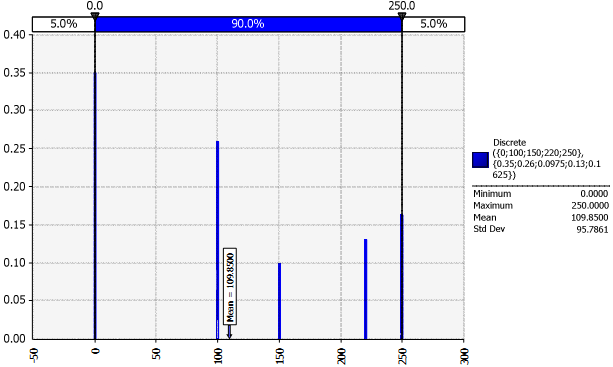
Example (Risk 3)
A project team is contemplating a geotechnical risk of the land on which a new hospital will be built. There is a 65 per cent probability that the soil is unstable and that some areas will need pre-treatment before construction can begin. Given that soil is unstable, the engineers have estimated that there is:
• A 40 per cent chance that one area needs to be fixed at the cost of $100,
• A 15 per cent chance that two areas need to be fixed at the cost of $150,
• A 20 per cent chance that three areas need to be fixed at the cost of $220, and
• A 25 per cent chance that four areas need to be fixed at the cost of $250.
The expected value of geotechnical risk is $109.85, calculated as follows:
= 65% x { 40%($100) + 15%($150) + 20%($220) + 25%($250)} = $109.85
The discrete distribution for this example is shown in Figure 13. The figure shows that this distribution has two peaks and the most likely outcome will be somewhere around $100.
Figure 13: Discrete distribution of Risk 3