2.5  Monte Carlo Analysis

Monte Carlo analysis is an analytical technique in which a large number of simulations are run using random quantities for uncertain variables and looking at the distribution of results to infer which values are most likely.

Monte Carlo analysis overcomes significant limitations of both traditional sensitivity analysis and discrete analysis, which typically becomes very cumbersome beyond two model input variables. Monte Carlo analysis, on the other hand, can accommodate an almost unlimited number of input variables, and allows the overall effect to be observed on the desired outcomes. The sensitivity of one input on the outcome can still be measured and improvements relating to better measure of variability can be made. Monte Carlo analysis also allows the individual effects of each simulated input to be ranked according to their affect on the outcome relative to the other simulated inputs.

Monte Carlo simulation assigns a range of potential input values to each input variable. These input values can be based on a discrete analysis, outputs from a probability distribution, or direct user inputs (effectively a custom probability distribution). An output (or range of outputs) is defined before the simulation is run.

The Monte Carlo simulation runs 'trials' of the model a specified number of times (usually 10,000 or more). For each trial the simulation chooses and new input for each of the variable inputs according to the distribution selected for that input. The model is then calculated and the output result is logged. When all the trials are complete the range of results is available for statistical testing or display.

In order to show the values of risks and the whole cost of the public sector comparator and Shadow Bid as a range, it is essential to perform a Monte Carlo distribution. Figure 16 shows the range of costs for a PSC and a DBFO delivery model. In this figure the mean value for the cost of the DBFO is $70 million less than the PSC, indicating positive value for taxpayers.

Figure 16:  Overlay distribution of total PSC costs and DBFO costs

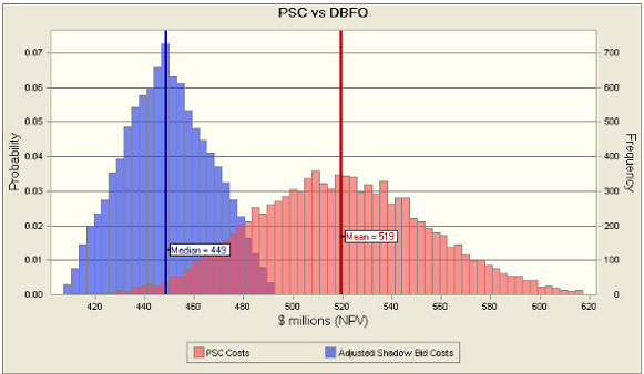
Generating the distribution for the PSC is relatively easy as there is no financing in the PSC. However, generating the distribution for the Shadow Bid, assuming it involves financing, is more complicated. A useful simplification is to determine the three points on the distribution that include:

●  The expected value

●  Five per cent value

●  Ninety-five per cent value

For each of these three points the model will have to be re-optimized but once obtained, the distribution can be generated very easily.

The $70 million in value for money demonstrated in Figure 16 is based on comparing the means of the two distributions. The mean of the distribution can also be referred to as the P50 value, as 50 per cent of the values under the curve lie above and below the P50 value. Partnerships BC has used a range of P values from P50 to P85 depending on the amount and quality of information available to the project team. The project team needs to justify any level other than P50. As Partnerships BC has moved towards establishing a pass/fail affordability ceiling as its guidance, it is imperative that the correct value be chosen to calculate the affordability ceiling, otherwise bidders will be unduly eliminated and/or the scope of the project (and benefits) will have to be reduced.