Types of probability distributions

There are a large number of probability distributions that may be used, the most common distributions other than the normal distribution are:

■ Binomial distribution. Returns the number of successes within in a given sample size where each trial has a probability p of success. The binomial distribution uses a Bernoulli process, which involves a sequence of trials where there are only two possible outcomes, for example the probability that a certain value will be observed from a random sample of a large population, based upon a fixed probability for that value.

■ Poisson distribution. Describes the number of independent events that will occur per unit of time where the rate of occurrences is constant but unlimited. The Poisson distribution may be useful as means to establish a performance measurement system. For example, the Poisson distribution returns the cumulative probability of a given number of failures occurring against an average or expected number of failures.

■ Uniform distribution. Applies where the variables are bounded by maximum and minimum values, but all variables have an equal likelihood of occurrence.

■ The triangular distribution is characterised by a minimum, most likely and maximum value and is used when there are reasonable grounds for believing that the probability distribution is not normal. The triangular distribution is useful when analysing cost behaviour relating to construction, maintenance and operations, where large cost overruns can happen, but with relatively low probability. The triangular distribution allows for a reasonably accurate calculation of contingency costs that must be included in the PSC. In the absence of evidence to the contrary, project risks should be assumed to follow a triangular distribution.

Figure 2: Right-tailed triangular distribution

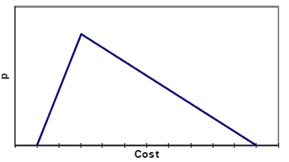
It should be noted that in a triangular distribution the mean or expected value is not the most likely value, but is given by:

[Minimum + most probable + maximum]/3

Example

A project team is considering the residual value of risk of light rail rolling stock, initial costing $100 million, after 20 years use. The residual value of the rolling stock is a function of a range of factors such as usage intensity, quality of maintenance and technological obsolescence. Lacking comprehensive historical data, the project team believes that the distribution of possible values is in the form of a triangular distribution, based on the logical assumption that the rolling stock is unlikely to fetch very high values, but there is a reasonable prospect of very low resale values. The likely range of values is:

The expected residual value is roundly $15 million, which should be reflected in the PSC, not the forecast value ($20 million). However, there is no information on the extent to which the actual residual value may vary. Random sampling of the distribution using as utility such as @Risk provides the following distribution

Figure 3 Triangular distribution of residual values

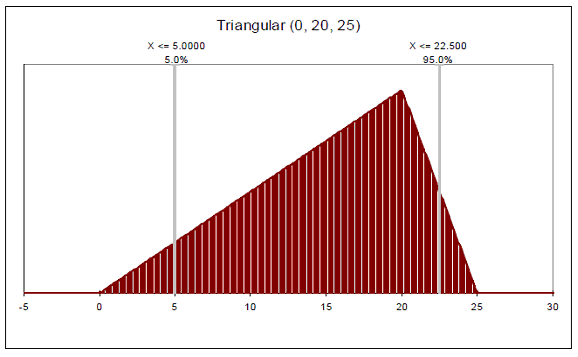
The project team may wish to make a further risk adjustment in view of the extreme "tail" of the distribution. An appropriate adjustment may be to take the 50th percentile ($12.5 million). The PSC would record an expected receipt of $15 million, with a downward risk adjustment of $2.5 million.