8.2 Valuing Retained Risk

Valuing Retained Risk represents the final stage in the construction of a PSC. This process can be summarised in the following steps:

Figure 8-2 Steps in valuing Retained Risk

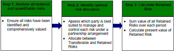
Step 1 (analyse all material and quantifiable risks) builds on the general risk valuation methodology provided in Section 6.2. Again it should be emphasised that all material risks need to be identified and valued before considering allocation issues. Practitioners are encouraged to revisit Section 8.2 as required to supplement their understanding of this process of valuing Retained Risk.

Step 2 (identify optimal risk allocation) is addressed in Section 7 as part of determining the optimal risk allocation for the purposes of valuing Transferred Risk and Step 3 (calculate Retained Risk) is dealt with in this Section 8.

Although the types of risk that should be borne by government need to be assessed individually for each project, Retained Risk may typically include:

• state change in law risk;

• the portion of commissioning or defect risks that may be caused by flaws in the output specification; and

• the portion of demand risk which government may assume, for example if the output specification contains a base level of demand.

Government may generally be suited to managing parts of state change in law risk due to its unique understanding and role in the regulatory process. Valuing change in law risk first requires an assessment of the impact of the key regulations/legislation influencing a project, and the likely impact of changes to the current regulatory framework. In the short term, for example, government may be better able to manage changes to the regulatory environment over which it has jurisdiction (i.e. Australian State laws and regulations). Change in law risk is discussed further in Risk Allocation and Standard Commercial Principles.

There may also be additional risks that government agrees to take for policy or other reasons. This recognises the particular responsibilities and accountabilities of government with respect to the delivery of services to the community.

Once all the Retained Risks have been identified, the size and timing of the expected cash flows associated with each of these risks needs to be aggregated to determine the NPC of the Retained Risk component of the PSC. Each of the risks should be included as a separate cash flow item and then added to form the Retained Risk component to allow for a detailed analysis of the key risks and their sensitivity to the overall PSC.

Example 3 Valuing Retained Risk

Consider the project for the provision of a new educational facility and related ancillary services discussed in Example 2 (Section 7.2). Again, the project risks have been allocated as shown in Table 8-1.

Table 8-1 Simplified risk allocation
Risk	Transferred Risk	Retained Risk
Design and construction risk	x
Change in law risk		x
Operating risk	x
Demand risk • base level demand • additional usage*	x	x
Maintenance risk	x
Security risk (e.g. vandalism) • during school hours • after school hours	x	x
Technology risk (e.g. computers)	x

	*Includes any potential third-party revenue risk
For the first five years of the project, the real periodic cash flows for the Retained Risk component of the PSC may look something like Table 8-2.

Table 8-2 Retained Risk cash flow valuation - real flows
Cost	Year 0 ($m)	Year 1 ($m)	Year 2 ($m)	Year 3 ($m)	Year 4 ($m)	Year 5 ($m)
Change in law risk		0.5	1.0	2.0	3.0	3.0
Demand risk
• base level demand		0.5	0.5	0.5	0.5	0.5
Security risk (e.g. vandalism)
• during school hours		1.0	1.0	1.0	1.0	1.0

Note that the financial impact of change in law risk increases over time, due to increasing uncertainty in the future (e.g. changes to wheelchair or other access requirements, or an increase in safety obligations that may require alterations to the facilities).

The effects of expected inflation (or appropriate cost index) are added to give the appropriate periodic cash flows and are then discounted to give the present value of Retained Risk for the project. In Table 8-3, all costs are inflated at 2.5 per cent per year.

Table 8-3 Retained Risk cash flow valuation - nominal flows
Cost	Year 0 ($m)	Year 1 ($m)	Year 2 ($m)	Year 3 ($m)	Year 4 ($m)	Year 5 ($m)
Change in law risk		0.5	1.1	2.2	3.3	3.4
Demand risk
• base level demand		0.5	0.5	0.5	0.6	0.6
Security risk (e.g. vandalism) • during school hours		1.1	1.1	1.1	1.1	1.1
Total Retained Risk	0.0	2.1	2.7	3.8	5.0	5.1
Discount factor @ 8.65% p.a. (assumed)	1.00	1.09	1.18	1.28	1.39	1.51
Discounted cash flows	0.0	2.0	2.3	3.0	3.6	3.4
Present value	14.3

In the above example, the value of Retained Risk is $14.3 million. The total value of risk in the PSC is therefore $91.0 million (including $76.7 million for Transferred Risk).